Remote Sensing Lab 4: Miscellaneous Image Functions

Goal and Background:

The goal of this lab is to gain the skills and knowledge about seven different miscellaneous image functions:

1). Utilizing the Inquire box or delineating an Area of Interest (AOI) to create an image subset.

2). Optimize the image spatial resolution by creating a higher spatial resolution image from a coarse        resolution image.

3). Introduction to the radiometric enhancement techniques.

4). Familiarizing linking a satellite image to Google Earth.

5). Introduction to resampling techniques.

6). Exploring the process of image mosaicking.

7). Introduction to binary change detection with simple graphic modeling.

Methods:

ERDAS Imagine was used to complete each of the following tasks.

1). Image Subsetting of a Study Area:

If the size of the satellite image you are working with is much larger than your study area or AOI, you can subset the area that you want so only that specific area is shown in the viewer. One method to create a subset is by using the Inquire box (Figure 1). With an image already in the viewer, add an Inquire box on the image. Adjust the size and location so that the Inquire box covers the AOI. Next, under the Raster tab, select the Subset and Chip tool and go to Create Subset Image. Save the image in the appropriate output folder and make sure to click From Inquire Box from the Subset widow to ensure the coordinates of the image will match with the Inquire box. The next method is to create a subset by using an AOI shape file. With an image already in the viewer, add the AOI shape file in the same viewer. Then select the shape file so that it is highlighted. After that, click on the Home button and select paste from selected object. Dotted lines will appear indicating that an AOI was created from the shapefile (Figure 2). Lastly, save the AOI as an AOI file, and once again select Subset and Chip from Raster tools to create the subset image and then save.

Figure 1: Subset using Inquire Box

Figure 2: Dotted lines indicating the AOI was created from the shape file. 

2). Image Fusion:

With the desired images already in the viewers, select the Raster tools and go to Pan Sharpen and then Resolution Merge (Figure 3). Once the Resolution Merge window is open, set the methods to Multiplicative and the resampling techniques to Nearest Neighbor. Lastly, save in the appropriate output folder.

Figure 3: Both Images Before the Resolution Merge

3). Simple Radiometric Sampling Techniques:

With the desired image already in the viewer (Figure 4), select Raster and go to Radiometric and then Haze Reduction. Input the correct image and then save to the appropriate output folder.

Figure 4: Image Before Haze Reduction

4). Linking Image Viewer to Google Earth:

With the desired image already in the viewer (Figure 5), select Connect to Google Earth. Next, click Match GE to View to have the image viewer and the Google Earth window be at the same extent. To synchronize both windows, select Sync GE to View (Figure 6). Google Earth aids as a selective interpretation key.

Figure 5: Image

Figure 6: Google Earth

5). Resampling:

There will be two sampling techniques in this section. First, with the desired image already in the viewer, select Raster and go to Spatial and then Resample Pixel Size. Set the resampling method to Nearest Neighbor and change the output cell size from 30x30 meters to 15x15 meters. Finally, check the Square Cells box to ensure that the output pixels will be square. Second, repeat the same process as previously but set the sampling method to Bilinear Interpolation.

6). Image Mosaicking:

This image function is useful when the AOI is divided between two images. There are two different ways to mosaic images together. First, add two images into the same viewer but make sure that Multiple Images in Virtual Mosaic is checked before adding them (Figure 7). Next, select Raster and go to Mosaic and then Mosaic Express. For the second method, add two images in the same viewer, select Raster and go to Mosaic and then MosaicPro. Once the MosaicPro window is open, add one of images in and click the Compute Active Area. Then add the second image in and do the same. Open the Color Corrections window and check the Use Histogram Matching box and then select the Set button. This will take you to the Histogram Matching pop up window where the Matching Method will be changed to Overlap areas.

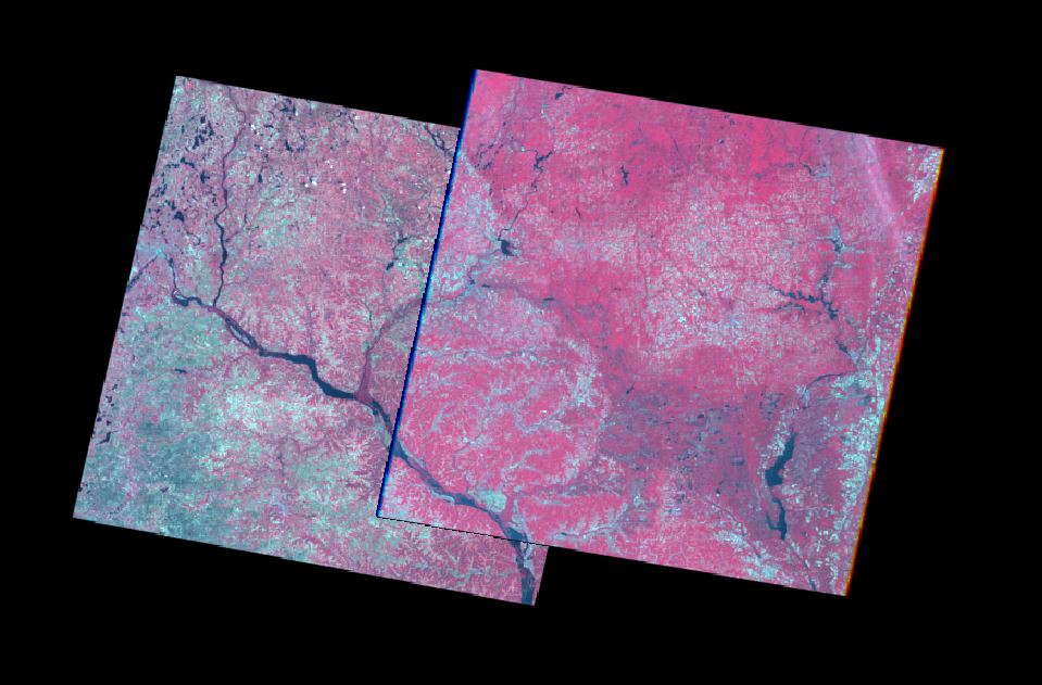Figure 7: Two Overlapped Images Before Mosaic

7). Binary Change Detection:

First, add two viewers and add the desired images, one in each viewer. Select Raster and go to Functions and then Two Image Functions. Change the operator from + to -. After the image differencing has ran, bring the new image into a viewer and view the metadata. The image does not display the difference but by looking at the histogram, a cut off point can be determined by using a rule of thumb threshold of mean + (1.5) Standard Deviation. Model Maker can also be used to show change by completing the same process (Figure 8). After the Model Maker has run the process, the resulting raster image was opened in ArcMap to show the change through a map.

Figure 8: Example of Operation Completed by Model Maker

Results:

1). Image Subsetting of a Study Area: The results of subsetting an area using the Inqurie Box (Figure 9)  method and the AOI shape file method(Figure 10). 

Figure 9: Inquire Box Method

Figure 10: AOI Shape File Method 

3). Simple Radiometric Sampling Techniques: Image after Haze Reduction (Figure 11).

Figure 11: Image After Haze Reduction

5). Resampling: Result of images after the Bilinear Interpolation (Figure 12) resampling technique and the Nearest Neighbor (Figure 13) resampling technique. With both Figure 12 and Figure 13, the original image is on the left and the resampled image is on the right. 

Figure 12: Bilinear Interpolation Technique

Figure 13: Nearest Neighbor Technique

6). Image Mosaicking: The result images from Mosaic Express (Figure 14) and MosaicPro (Figure 15). 

Figure 14: Result from Mosaic Express

Figure 15: Result from MosaicPro

7). Binary Change Detection: The histogram with the cut off points (Figure 16), along with the map (Figure 17) that shows the changed areas from 1991 to 2011. 

Figure:16 Histogram With Cut Off Points

Figure 17: Map Representing Changed Areas

Sources:

Images and data provided by my professor and the Geography Department of the University of Wisconsin-Eau Claire. ERDAS Imagine and ArcMap were used to complete this lab.