Remote Sensing Lab 6: Geometric Correction

Goal and Background:

The goal of this lab was to introduce geometric correction. This lab covered two major types of geometric correction. These correction types are usually used for satellite images as part of the preprocessing activities prior to the extraction of biophysical sociocultural information from satellite images. During the process of this lab, a United States Geological Survey 7.5 minute digital raster graphic image of the Chicago Metropolitan Statistical Area was used to collect ground control points (GCPs). Additionally, a corrected Landsat TM image for eastern Sierra Leone was used to rectify a geometrically distorted image.

Methods:

Erdas Imagine was used to complete this lab.

Part One: Image-to-Map Rectification

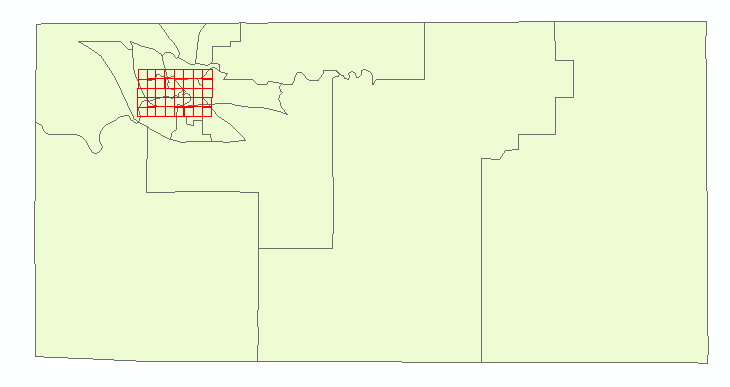
In the first part of the lab, a USGS 7.5 minute digital raster graphic image (Chicago_drg.img) of the Chicago region was added to one viewer and then another Chicago region image (Chicago_2000.img) was added to the second viewer. The Chicago_2000.img was highlighted because that was the image that was going to be rectified. Next, Multispectral was selected and the Control Points were clicked. This activated the Multipoint Geometric Connection window. The next task is to start adding the GCPs to the images, but the default GCPs need to be deleted first. In this process, a first order polynomial transformation was performed so there needed to be at least three pairs of GCPs. However, four pairs were added to ensure that the output image would have a good fit. To perform this task, the Create GCP tool was selected and the first GCP points were added to the Chicago_drg.img and the Chicago_2000.img. To display the reference coordinates easier over the images, the color of the points was changed to purple. Three more GCP points were added to the image to have a total of four. To ensure the accuracy of the GCPs, the Root Mean Square (RMS) error should be 2.0 or below for part one (Figure 1). The GCPs were repositioned multiple times to try and achieve total accuracy. Once the RMS error was below 2.0, the Display Resample Image Dialogue tool was selected to perform the geometric correction. All of the parameters were left as default in the resample image window and the tool was run.

Figure 1: RMS Error Below 2.0 With 4 GCPs

Part Two: Image-to-Image Registration

In part two of the lab, two new images were added to separate viewers. One of the images (sierra_leone_east1991.img) has serious geometric distortion. The second image (sl_reference_image.img) is an already referenced image. The Swipe tool was used to show the contrast between the referenced image and the geometrically distorted image by moving the slider tab left and right (Figure 2).

Figure: Swipe Tool Showing the Contrast Between the Referenced Image and the Geometrically Distorted Image

Next, Multispectral was selected and the Control Points were clicked. Once again, the default GCPs were deleted. In part two, a third order polynomial transformation was performed so there needed to be at least ten pairs of GCPs. A total of 12 GCPs were added to ensure that the output image would have a good fit. To ensure the accuracy of the GCPs, the RMS error should be 0.5 or below this part because at this point there is some experience (Figure 3). The points were repositioned multiple times to achieve a low enough RMS error. Once the RMS error was 0.5 or below, the Display Resample Image Dialogue tool was selected to perform the geometric correction. All of the parameters were left as default in the resample image window and the tool was run.

Figure 3: RMS Error Below 0.5 With 12 GCPs

Results:

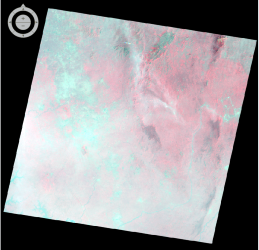
Figure 4 is the geometrically corrected image from part one after using the Display Resample Image Dialogue tool. This geometrically corrected image was the result of a USGS 7.5 minute raster digital raster graphic image of the Chicago region and then another Chicago region image. There was minimal distortion on the Chicago image so only a first order polynomial transformation was needed. A nearest neighbor resampling method was used used to complete the spatial interpolation.

Figure 4: Result of Geometrically Corrected Image Part One

Figure 5 is the geometrically corrected image from part two after using the Display Resample Image Dialogue tool. This geometrically corrected image was the result of an already reference image and a severely geometric distorted image. Since there was serious distortion on one of the images, a third order polynomial transformation was required. A bilinear resampling method was used used to complete the spatial interpolation.

Figure 5: Result of Geometrically Corrected Image Part Two

Figure 6 is showing the contrast between the original referenced image and the geometrically corrected image using the Swipe tool.

Figure 6:S wipe Tool Showing the Contrast Between the Original Referenced Image and the Geometrically Corrected Image

Sources:
Satellite images from Earth Resources Observation and Science Center, United States Geological Survey Digital raster graphic (DRG) from Illinois Geospatial Data Clearing House.  

Remote Sensing Lab 5: LiDAR Remote Sensing

Goal and Background:

The goal of this lab is to gain the skills and knowledge on LiDAR data structure and processing. This lab has two specific objectives. First, there will be processing and retrieval of various surface and terrain models. Second, there will be processing and creation of an intensity image and other derivative products from a point cloud. This lab will include work with LiDAR point clouds in a LAS file format. Understanding LiDAR processing is important in the field of remote sensing as it is experiencing a significant growth in job creation. 

Methods:

Erdas Imagine and ArcMap were used to complete this lab.

Part One: Point Cloud Visualization in Erdas Imagine:

In the first part of the lab, LiDAR point clouds were opened in Erdas Imagine. Each LAS file was examined to determine whether there was an overlap of points at the boundaries of tiles. Two important facts that should be retrieved from the data are the metadata and the tile index. The tile index file was then opened in ArcMap to be viewed.

Part Two: Generate a LAS dataset and explore lidar point clouds with ArcGIS:

The first step in this process was to open ArcMap and create a LAS Dataset from the LAS folder and name it Eau_Claire_City.lasd. Next, the LAS Dataset Properties window was opened and all of the necessary LAS files were added. After that, the Statistics tab was selected and the statistics were calculated (Figure 1). Once the statistics were calculated, an assigned coordinate system was chosen in the XY Coordinate System tab. For this lab, the Nad 1983 HARN Wisconsin CRS Eau Claire (US FEET) was most appropriate. After that, the Z Coordinate System tab was selected. NAVD 1988 US feet was chosen for the vertical coordinate system.

Figure 1: Eau_Claire_City.lasd Statistics

Eau_Claire_City.lasd can now be displayed. Eau_Claire_City.lasd appeared as a LAS Dataset tiles with red boundaries. So, a shapefile of Eau Claire County was added to the layout to confirm that the LAS Dataset was spatially located correctly (Figure 2). The data from the LAS Dataset would not display until zoomed in to a specific tile. For the points to show, the Layer Properties Window needed to be opened to the Symbology tab. Once there, the natural breaks was set to 8 classes.

Figure 2: The Eau Claire County Shapefile with the Eau_Claire_City.lasd.

The different Classification Codes and Returns were examined and familiarized. Additionally, the LAS Dataset Profile View tool was used to examine the side profile of a bridge in point cloud form (Figure 3). This tool was used as an aid in visualization.

Figure 3: The Side Profile of a Bridge Using the LAS Dataset Profile View tool

Part Three: Generation of LiDAR Derivative Products

Section 1: Deriving DSM and DTM Products From Point Clouds

The first product that was generated was a Digital Surface Model (DSM). The layer was set to display Points by elevation and filtered to First Returns. Before creating the derivative product, the LAS Dataset needed to be converted to a raster output. This was done by utilizing the LAS Dataset to Raster tool. The sampling type was set to cellsize and the sampling value was set to 6.56168 (2 meters). The measuring tool was used to confirm that the cell size of the output raster was 2 meters. To enhance the DSM, a hillshade was created using the Hillshade tool.  6.56168

The second product that was generated was a Digital Terrain Model (DTM). The layer was set to display Points by elevation but this time it was filtered to Ground. Once again, the LAS Dataset to Raster tool was used. The sampling type was set to cellsize and the sampling value was set to 6.56168 (2 meters). After the DTM was created, the Hillshade tool was used again to enhance the DTM.

Section 2: Deriving LiDAR Intensity Image From Point Cloud

In this section, a LiDAR intensity image was generated. The layer was used again set to display Points by elevation and filtered to First Returns. The LAS Dataset to Raster tool was also used again except the value field was set to Intensity. The output image was then opened in Erdas Imagine for a more enhanced display.

Results:

Figure 4 is the output DSM from the LAS Dataset to Raster tool using the First Return filter. The lighter and darker grays show difference in elevation with the lighter grays displaying a high elevation and the darker grays displaying a low elevation. DSM's include buildings and vegetation on the surface.

Figure 4: DSM 

Figure 5 is the output Hillshade of the DSM. The hillshade enhances the DSM by displaying a 3D representation of the surface. Buildings and vegetation are clearly seen on the Hillshade created from the DSM. This type of hillshade would be useful when analyzing any features that reside on top of earths surface. 

 Figure 5: DSM Hillshade

Figure 6 is the output DTM from the LAS Dataset to Raster tool using the Ground filter. The lighter and darker grays show difference in elevation with the lighter grays displaying a high elevation and the darker grays displaying a low elevation. DTM's include the bare earth surface.

Figure 6: DTM

Figure 7 is the output Hillshade of the DTM. The hillshade enhances the DTM by displaying a 3D representation of the surface. Because the DTM Hillshade is just displaying the bare earth surface, less detail is shown compared to the DSM Hillshade. This type of hillshade would be useful when analyzing the true elevation of the earths surface. 

Figure 7: DTM Hillshade 

Figure 8 is the intensity image displayed in ArcMap. The image appears very dark and it is hard to distinguish between objects.

Figure 8: Intensity Image Displayed in ArcMap

Figure 9 is the intensity image displayed in Erdas Imagine. The image is now enhanced and is much brighter and clearer. Objects can be identified and spatial connections can be made.

Figure 9: Intensity Image Displayed in Erdas Imagine

Sources:

LiDAR point cloud and tile index from Eau Claire County, 2013.