Remote Sensing Lab 5: LiDAR Remote Sensing

Goal and Background:

The goal of this lab is to gain the skills and knowledge on LiDAR data structure and processing. This lab has two specific objectives. First, there will be processing and retrieval of various surface and terrain models. Second, there will be processing and creation of an intensity image and other derivative products from a point cloud. This lab will include work with LiDAR point clouds in a LAS file format. Understanding LiDAR processing is important in the field of remote sensing as it is experiencing a significant growth in job creation. 

Methods:

Erdas Imagine and ArcMap were used to complete this lab.

Part One: Point Cloud Visualization in Erdas Imagine:

In the first part of the lab, LiDAR point clouds were opened in Erdas Imagine. Each LAS file was examined to determine whether there was an overlap of points at the boundaries of tiles. Two important facts that should be retrieved from the data are the metadata and the tile index. The tile index file was then opened in ArcMap to be viewed.

Part Two: Generate a LAS dataset and explore lidar point clouds with ArcGIS:

The first step in this process was to open ArcMap and create a LAS Dataset from the LAS folder and name it Eau_Claire_City.lasd. Next, the LAS Dataset Properties window was opened and all of the necessary LAS files were added. After that, the Statistics tab was selected and the statistics were calculated (Figure 1). Once the statistics were calculated, an assigned coordinate system was chosen in the XY Coordinate System tab. For this lab, the Nad 1983 HARN Wisconsin CRS Eau Claire (US FEET) was most appropriate. After that, the Z Coordinate System tab was selected. NAVD 1988 US feet was chosen for the vertical coordinate system.

Figure 1: Eau_Claire_City.lasd Statistics

Eau_Claire_City.lasd can now be displayed. Eau_Claire_City.lasd appeared as a LAS Dataset tiles with red boundaries. So, a shapefile of Eau Claire County was added to the layout to confirm that the LAS Dataset was spatially located correctly (Figure 2). The data from the LAS Dataset would not display until zoomed in to a specific tile. For the points to show, the Layer Properties Window needed to be opened to the Symbology tab. Once there, the natural breaks was set to 8 classes.

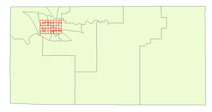Figure 2: The Eau Claire County Shapefile with the Eau_Claire_City.lasd.

The different Classification Codes and Returns were examined and familiarized. Additionally, the LAS Dataset Profile View tool was used to examine the side profile of a bridge in point cloud form (Figure 3). This tool was used as an aid in visualization.

Figure 3: The Side Profile of a Bridge Using the LAS Dataset Profile View tool

Part Three: Generation of LiDAR Derivative Products

Section 1: Deriving DSM and DTM Products From Point Clouds

The first product that was generated was a Digital Surface Model (DSM). The layer was set to display Points by elevation and filtered to First Returns. Before creating the derivative product, the LAS Dataset needed to be converted to a raster output. This was done by utilizing the LAS Dataset to Raster tool. The sampling type was set to cellsize and the sampling value was set to 6.56168 (2 meters). The measuring tool was used to confirm that the cell size of the output raster was 2 meters. To enhance the DSM, a hillshade was created using the Hillshade tool.  6.56168

The second product that was generated was a Digital Terrain Model (DTM). The layer was set to display Points by elevation but this time it was filtered to Ground. Once again, the LAS Dataset to Raster tool was used. The sampling type was set to cellsize and the sampling value was set to 6.56168 (2 meters). After the DTM was created, the Hillshade tool was used again to enhance the DTM.

Section 2: Deriving LiDAR Intensity Image From Point Cloud

In this section, a LiDAR intensity image was generated. The layer was used again set to display Points by elevation and filtered to First Returns. The LAS Dataset to Raster tool was also used again except the value field was set to Intensity. The output image was then opened in Erdas Imagine for a more enhanced display.

Results:

Figure 4 is the output DSM from the LAS Dataset to Raster tool using the First Return filter. The lighter and darker grays show difference in elevation with the lighter grays displaying a high elevation and the darker grays displaying a low elevation. DSM's include buildings and vegetation on the surface.

Figure 4: DSM 

Figure 5 is the output Hillshade of the DSM. The hillshade enhances the DSM by displaying a 3D representation of the surface. Buildings and vegetation are clearly seen on the Hillshade created from the DSM. This type of hillshade would be useful when analyzing any features that reside on top of earths surface. 

 Figure 5: DSM Hillshade

Figure 6 is the output DTM from the LAS Dataset to Raster tool using the Ground filter. The lighter and darker grays show difference in elevation with the lighter grays displaying a high elevation and the darker grays displaying a low elevation. DTM's include the bare earth surface.

Figure 6: DTM

Figure 7 is the output Hillshade of the DTM. The hillshade enhances the DTM by displaying a 3D representation of the surface. Because the DTM Hillshade is just displaying the bare earth surface, less detail is shown compared to the DSM Hillshade. This type of hillshade would be useful when analyzing the true elevation of the earths surface. 

Figure 7: DTM Hillshade 

Figure 8 is the intensity image displayed in ArcMap. The image appears very dark and it is hard to distinguish between objects.

Figure 8: Intensity Image Displayed in ArcMap

Figure 9 is the intensity image displayed in Erdas Imagine. The image is now enhanced and is much brighter and clearer. Objects can be identified and spatial connections can be made.

Figure 9: Intensity Image Displayed in Erdas Imagine

Sources:

LiDAR point cloud and tile index from Eau Claire County, 2013.